Inference in Bayesian Networks¶

Inference¶

Inference Problem:

Given: a Bayesian network
Given an assignment of values to some of the variables in the network: $E_i=e_i(i=1,\dots,l)$
- "Instantiation of the nodes $\bold E$ "
- "Evidence $\bold E=e$ entered"
- "Findings entered"
- ...
Want: for variables $A\notin \bold E$ the posterior margnial $P(A\mid \bold E=e)$

According to the definition of conditional probability, it is sufficient to compute for each $A\in D_A$ the value

$P(A=a,\bold E=e)$

Together with

$P(\bold E=e)=\sum_{a\in D_A}P(A=a,\bold E=e)$

This gives the posterior distribution

Inference as Summation¶

Let $A$ be the variable of interest, $\bold E$ the evidence variables, and $\bold Y=Y_1,\dots,Y_l$ the remaining variables in the network not belonging to $A\cup \bold E$ . Then

$$ P(A=a,\bold E=e)=\sum_{y_1\in D_{Y_1}}\cdots\sum_{y_l\in D_{Y_l}}P(A=a,\bold E=e,Y_1=y_1,\dots,Y_l=y_l) $$ Note:

For each $\bold y$ the probability $P(A=a,\bold E = \bold e, \bold Y = \bold y)$ can be computed from the network In time linear in the number of random variables
The number of configurations over $\bold Y$ is exponential in $l$

Inference Problems¶

First Problem¶

Find $P(B\mid a,f,g,h)={P(B,a,f,g,h)\over P(a,f,g,h)}$

We can if we have access to $P(A,B,C,D,E,F,G,H)$

$P(A,B,C,D,E,F,G,H)=P(A)P(B)P(C)P(D\mid A,B)\cdots P(H\mid E)$

Inserting evidence we get:

and

Second Problem¶

See naive solution in Lecture 14.10 Slides 8-11

Naive Solution Summary¶

Variable Elimination¶

Problem

The joint probability distribution will contain exponentially many entries

Idea

We can use

the form of the joint distribution $P$ , and
the law of distributivity

to make the computation of the sum more efficient

Thus, we can adapt our elimination procedure so that:

we marginalize out variables sequentially
when marginalizing out a particular variable $X$ , we only need to consider the factors involving $X$

Example¶

Factors¶

Calculus of factors

The procedure operates on factors: functions of subsets of variables
Required operations on factors:
- multiplication
- marginalization (summing out selected variables)
- restriction (setting selected variables to specific values)

Complexity

See example in Lecture 14.10 Slides 16-17

Singly Connected Networks¶

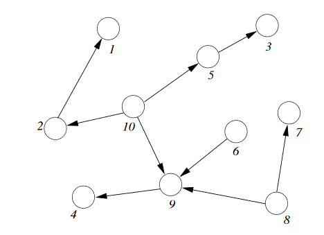
A singly connected network is a network in which any two nodes are connected by at most one path of undirected edges.

For singly connected network: any elimination order that "peels" variables from outside will only create factors of one variable.

The complexity of inference is therefore linear in the total size of the network ( = combined size of all conditional probability tables)

Approximate Inference¶

Sample Generator¶

Observation: can use Bayesian network as random generator that produces states $\bold X = \bold x$ according to distribution $P$ defined by the network